![]() TECTONICS BLOG
Rev. 2022-05-12
TECTONICS BLOG
Rev. 2022-05-12
|
Click on an image to enlarge it
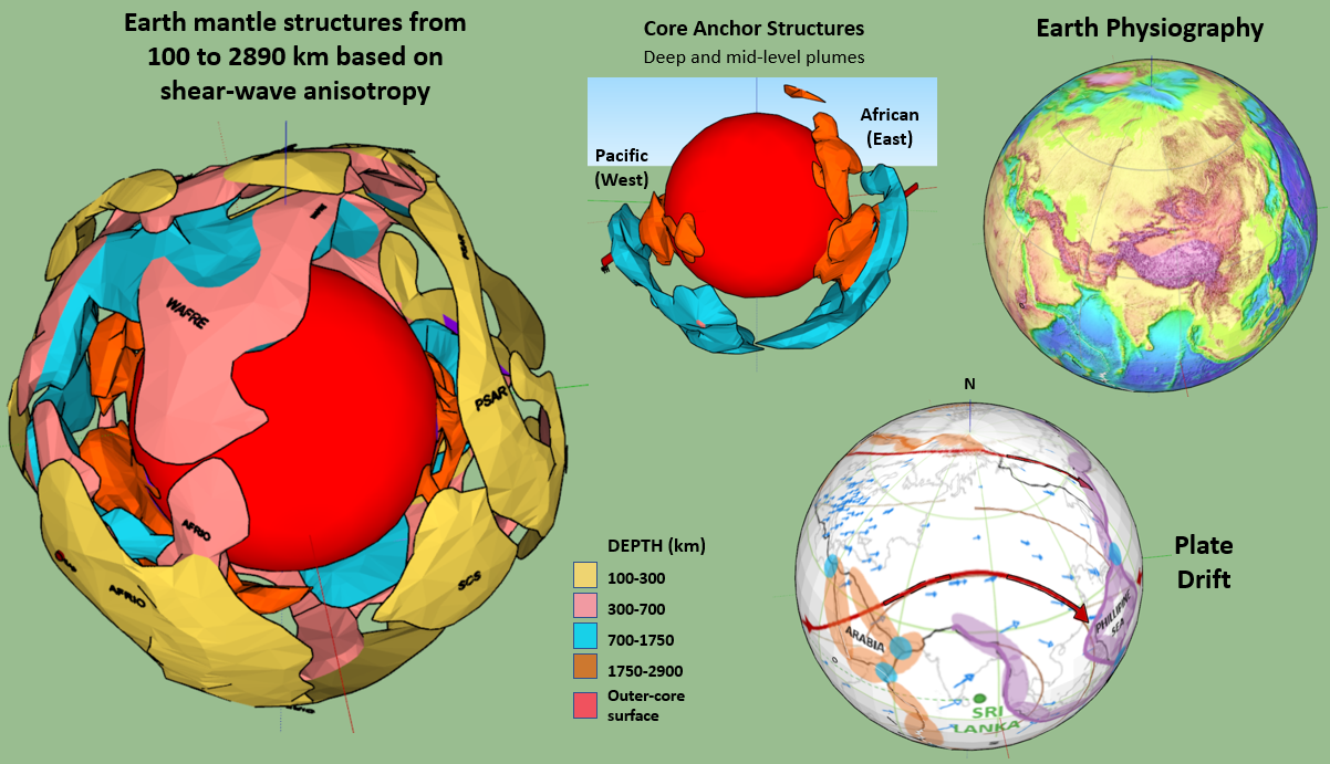
Figure 2. Various views of EarthCAD.ver.8.0.skp,
a SketchUp Pro 2020 model constructed using the slowest 35%
shear-wave, average velocities from the S362ANI+M S-wave velocity model (
Table 1. Average (Voigt) shear-wave velocities by depth and the mean - 15% values used to generate components for the solid-object, EarthCADv.8.0.skp model 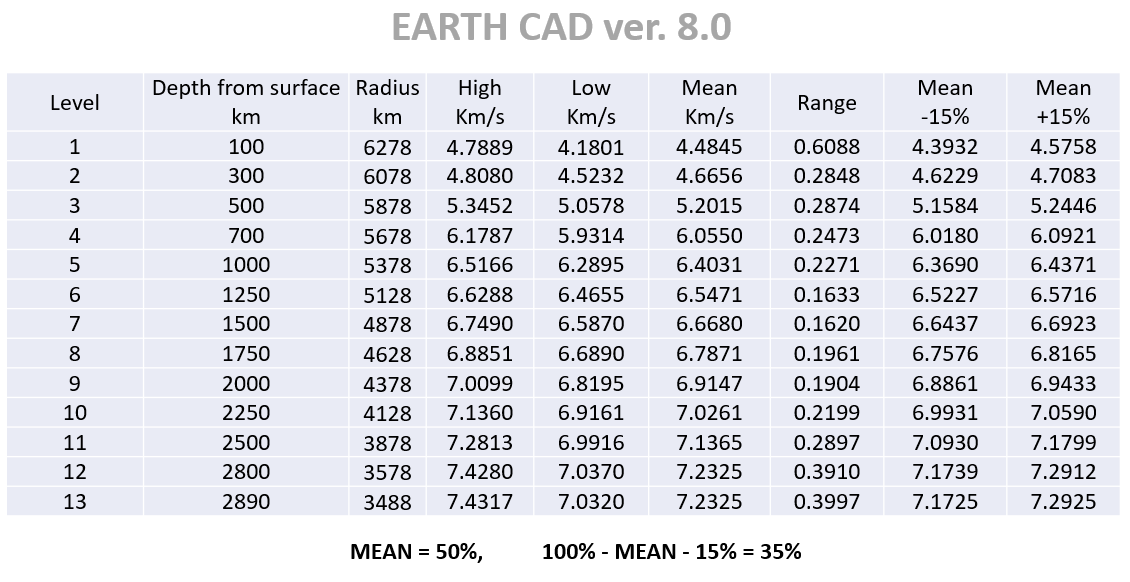 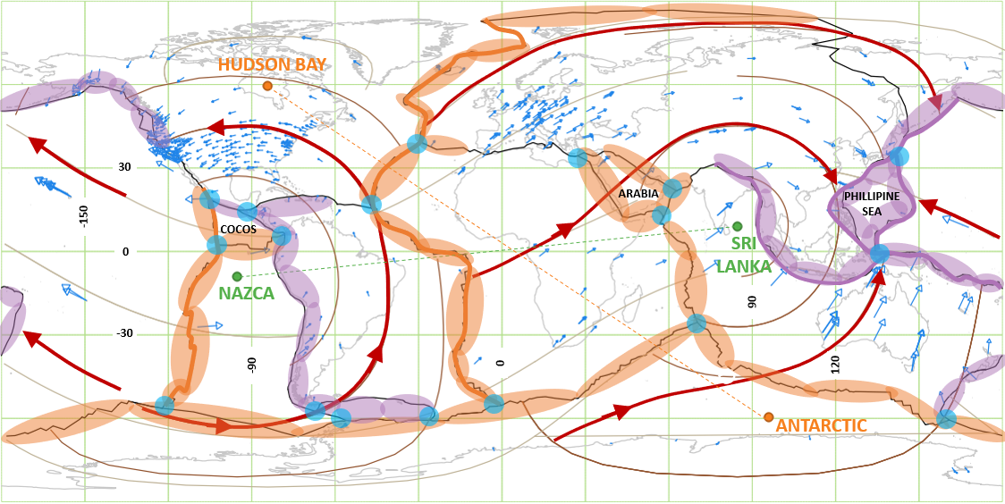
Figure 3.
Geographic map summarizing plate drift with respect to two dipoles
(Hudson Bay - Antarctica, and Nazca - Sri Lanka). The small, blue
vectors show locations of GPS ground stations, and the thick, red
vectors summarize plate drift following circles of expanding radii around each pole. The
Africa and Pacific plates are drifting along great circles about the Hudson Bay and
Antarctic dipole, but in
opposite directions. Motions of plates around these two poles generally
account for global-plate drift. Secondary perturbations follow great
circles around the Nazca
and Sri Lanka dipole. Purple ellipses are fit to subduction
trenches and orange ellipses highlight crustal spreading centers.
Plate triple junctions are highlighted blue.
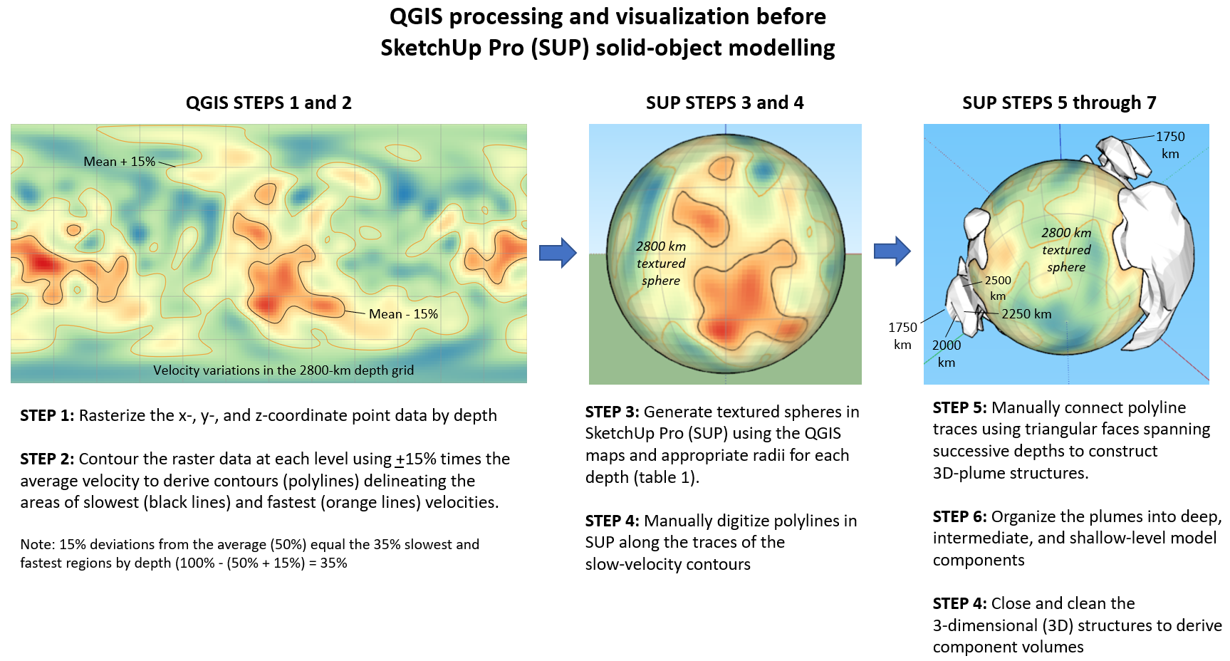 Figure 4. The 7-step process behind constructing EarthCAD.v.8.0.skp. 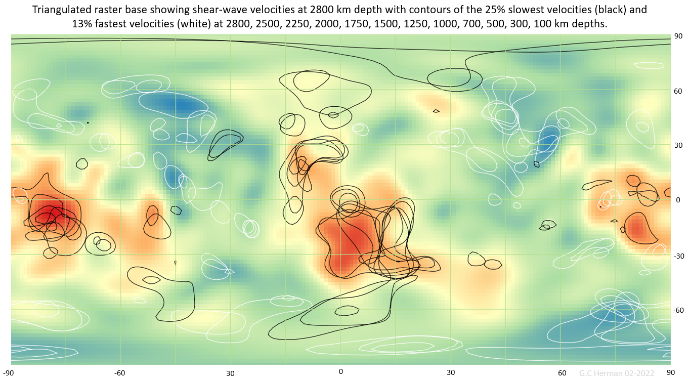 Figure 5. A geographic plot of mantle S-wave average velocities at 2800-km depth from Earth's surface, with equal-value contours (isopleths) generated along the 25% slowest (black lines) and the 13% fastest (white lines) values. The slow areas hypothetically define regions subject to convective mantle upwelling. Note the alternate banding of slow and fast regions trending from the lower right toward the upper left at the deepest mantle levels. 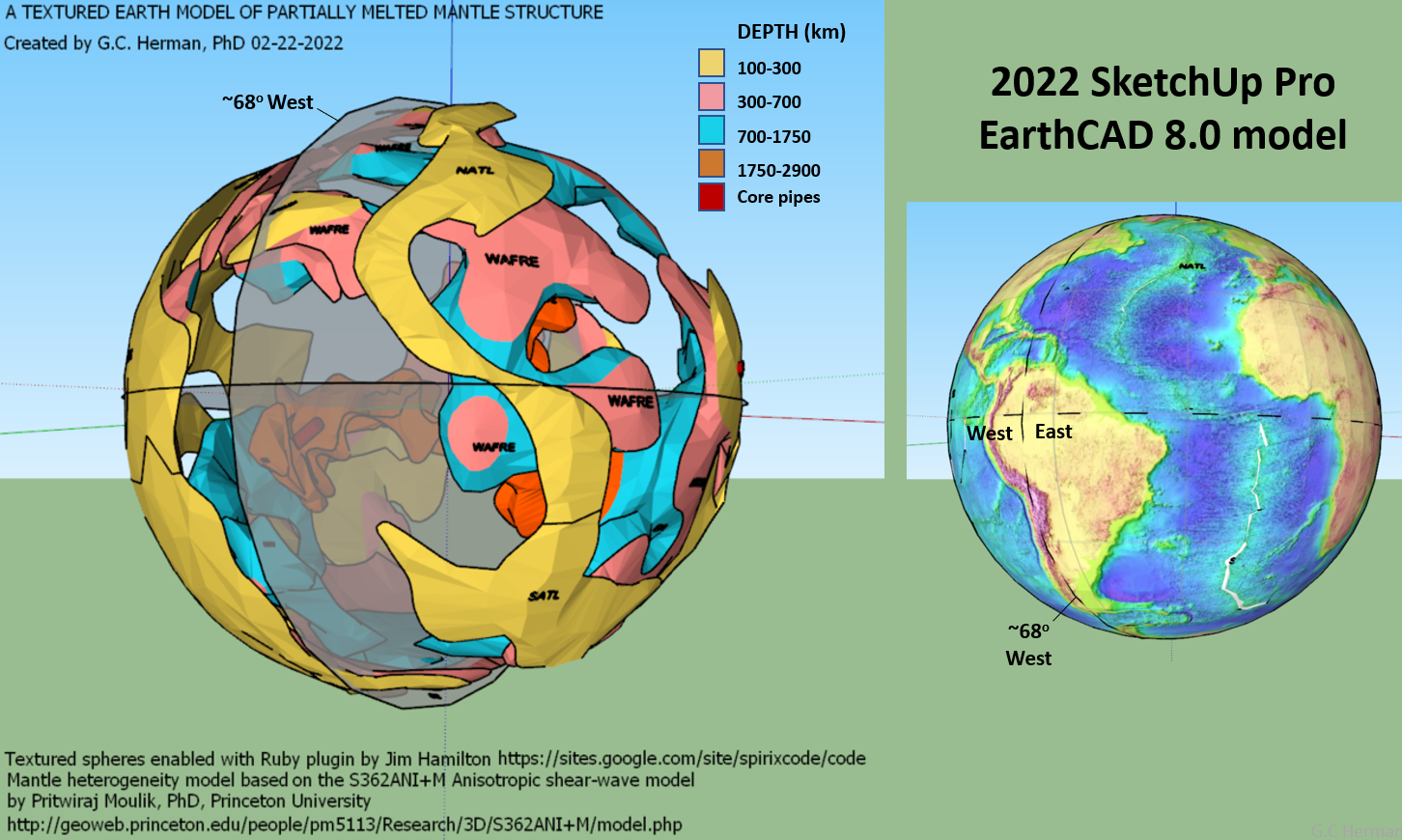 Figure 6. Two views of EarthCADv.8.0.skp . The left one shows the mantle plumbing with labeled sold-object component used for deriving volumes for hemispherical comparisons. 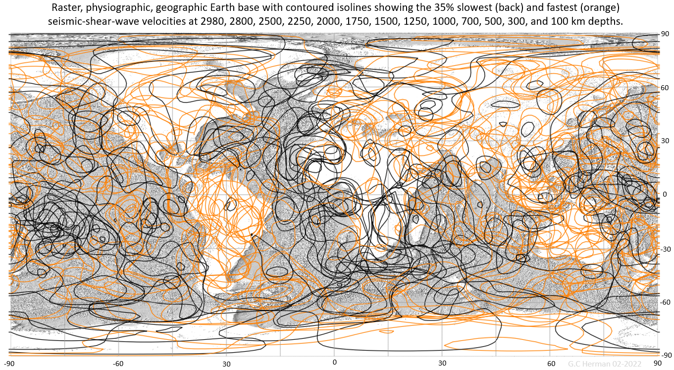 Figure 7. A geographic plot of the 35% slowest (black lines) and fastest (orange lines) S-wave, average mantle velocities average at 13 different depths below Earth's surface. Note the grouping of fast-velocity regions at all depth levels beneath many continents, and the tendency for the slowest-transmitted waves to occur in the oceanic realms. 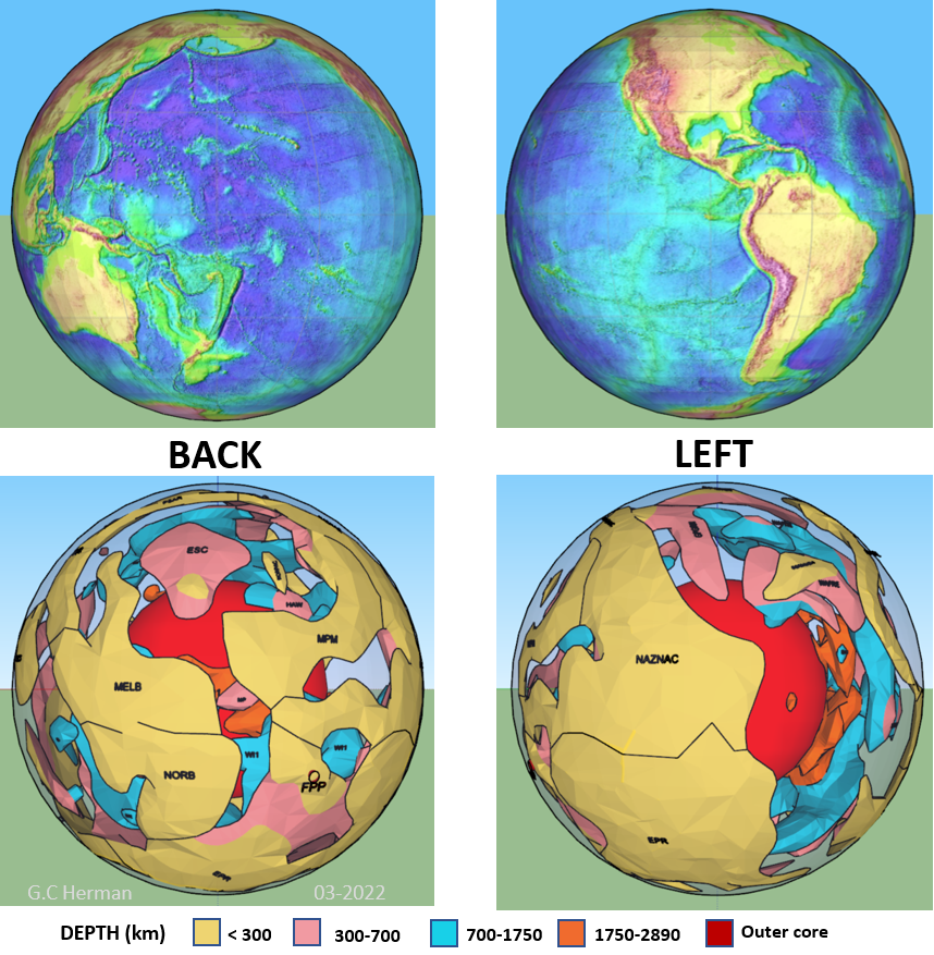 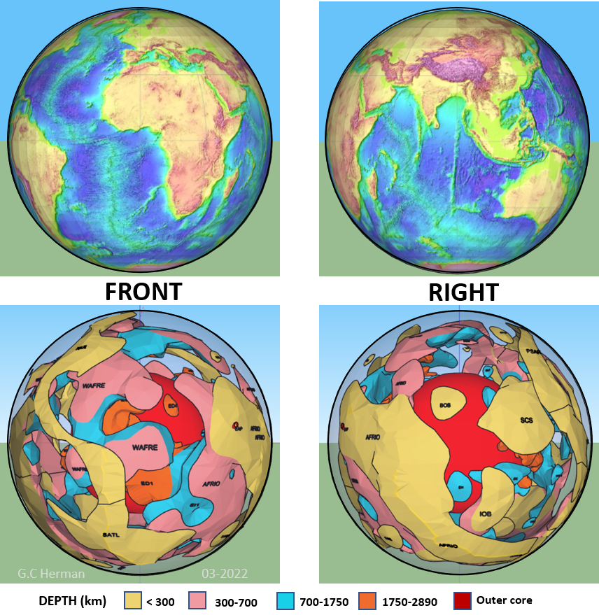 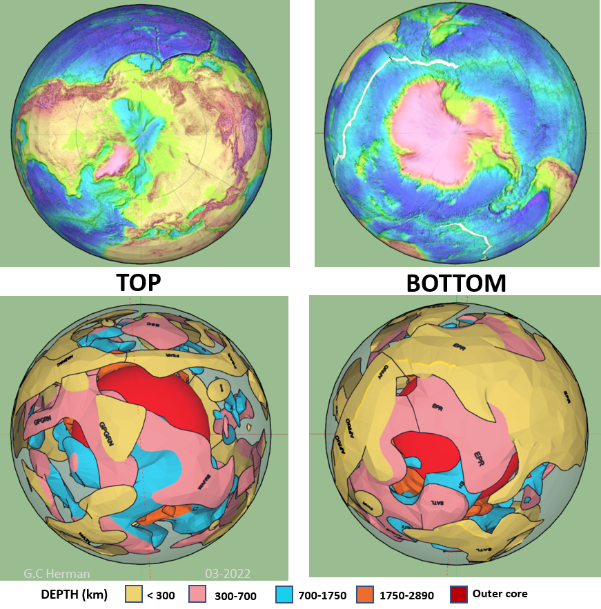 Figure 8. Six different model perspectives of EarthCADv.8.0.skp. 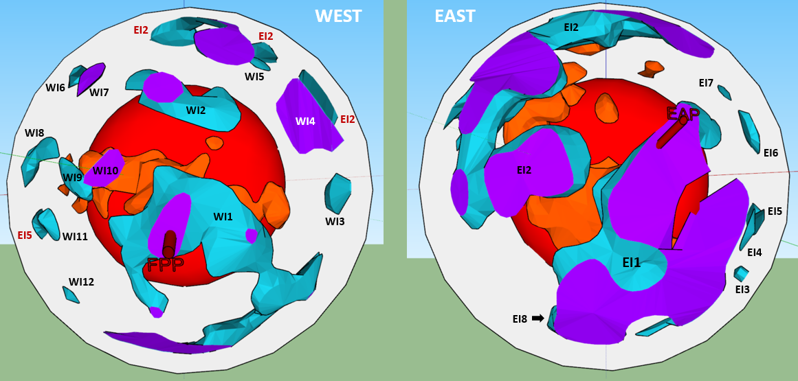 Figure 9. Hemisphere comparison of the deep and intermediate-level SVBs (>1750 km depth). Volumes of the labeled bodies are summarized in Table 2. The purple polygons are auxiliary 3D surfaces used to close bodies in order to attain volumes. This visual comparison of SVB volumes shows how the deep, eastern structures are three-time larger than their western counterparts. SVB colors are keyed above in figure 7. Table 2. Volumetric comparisons of connected and disconnected SVBs by hemisphere 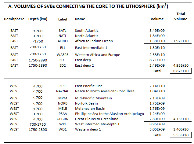 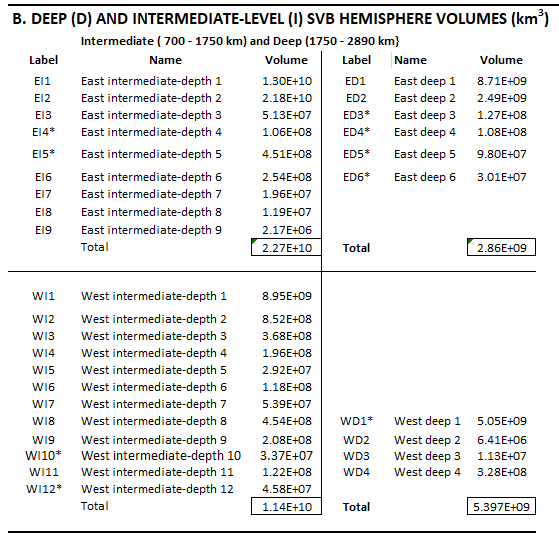 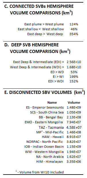 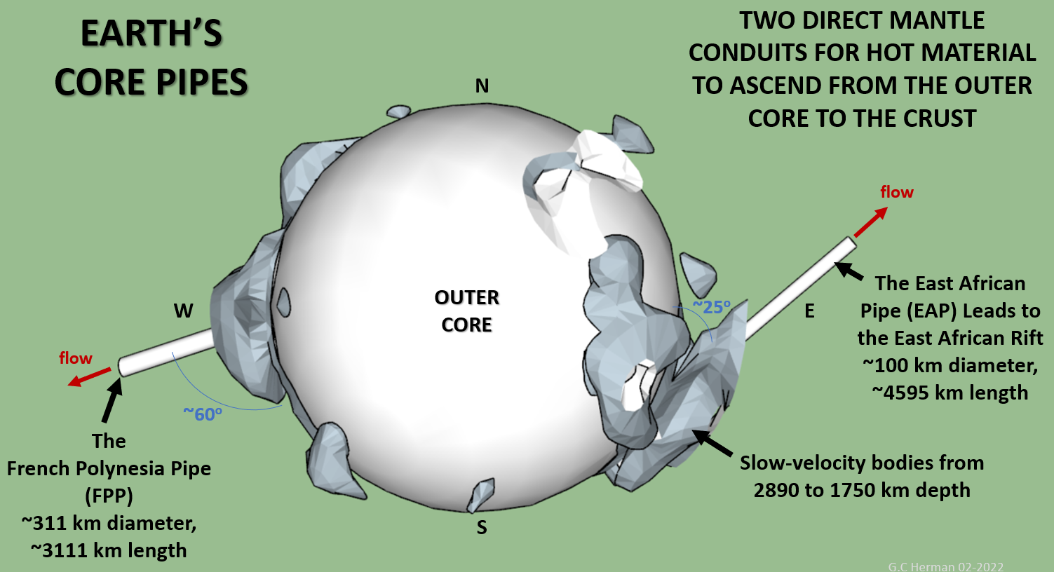 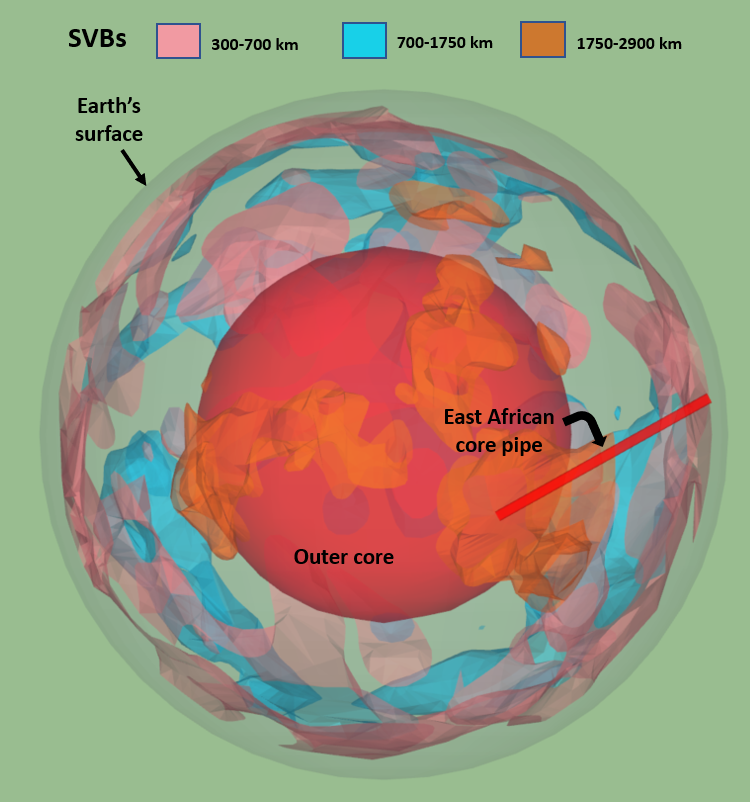 Figure 10. The CAD model reveals that there are two inclined pipelines rising directly from the outer core to Earth's lithosphere. The Eastern one leads to the East African Rift system and is fed by SVBs having over three times the volume of their counterpart in the Western hemisphere beneath the Pacific Ocean basin. 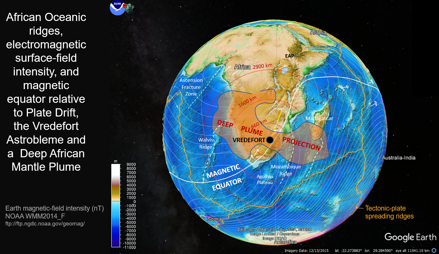 Figure 11. The South African region is where the deep plume rises off the outer core with likely roots stemming from the Proterozoic (2.023 Ga) Vredefort impact. It is likely that this event imparted structures that evolved into geodynamic components that continue to operate today. The spatial ties to Earth magnetic field supports the hypothesis that connected mantle plumes giving rise to Earth's poloidal magnetic-field component. Note that Earth's magnetic equator passes almost directly through the cratered region and the deep-mantle plume system that anchors overlying, connected bodies that traverse the mantle. Plate drift deflects along the same path as the magnetic equator. |
Gregory Charles Herman, PhD, Flemington, New Jersey, USA gcherman56@yahoo.com
The Vredefort astrobleme, mantle plumes, core pipes, and tectonic-plate drift
Two dipoles of plate drift * QGIS velocity data processing * SketchUp Pro EarthCADv.8.0.skp * Connected and disconnected SVBs * SVB volume analysis * Vredefort astrobleme, mantle structure and plate drift * The French Polynesia pipe * Relict planetary gneissic banding * Comments * References
Exploring life's inroads occasionally leads to fascinating, new discoveries. What began as an exercise to portray tectonic drift of the North American plate with a focus on the New York promontory, soon after evolved into a project of building a whole-Earth computer model suited for characterizing upward flowing plumes in the mantle. What emerged from the computer model is an unexpected discovery of the primary, motivating forces behind plate tectonics, and perhaps the reason that primates evolved in East Africa. These discoveries are shared in this illustrated article.
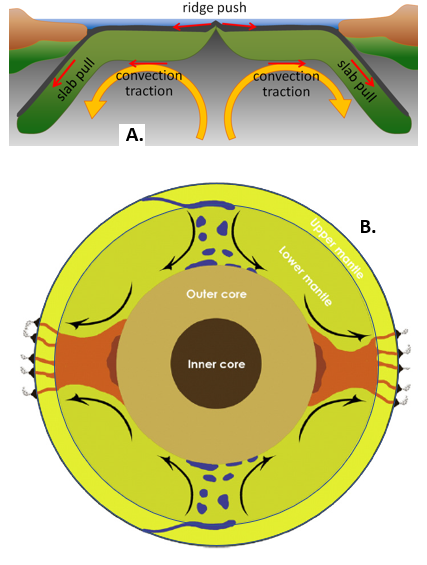
The forces driving Earth's tectonic plates to shift, rise, and sink can be difficult to fathom. Textbook explanations for the lateral forcing of plate movement, on average measuring about 25 millimeters of drift per year, include 1) ridge push, where new oceanic crust is continuously generated along diverging and relatively elevated oceanic ridges, 2) slab pull where old, thick, and relatively cold and dense oceanic crust dives steeply into the mantle along subduction zones owing to plate convergence, and 3) deep upwelling of hot, partially molten mantle material from depths reaching 2900 kilometers beneath Earth's surface at the core-mantle boundary (fig. 1). But which of these forces are the dominant ones? What forces are primarily responsible for continuously propelling the lithospheric plates around the planetary surface? In addition, after recognizing geodynamic effects stemming from the collision that made the Chicxulub impact crater (66 Ma; Herman, 2006), another question arises as to what strain effects large-bolide impacts have on lithospheric plate drift? Having spent the past few year developing CAD skills modeling three- (3D) and four-dimensional (4D) Earth and human systems, I knew the only place to seek the answers to such profound questions is in the realm of geophysical seismology. I had learned to characterize mantle structures using embedded 2D seismic tomography, and I wondered if there were more complete seismological data set for the mantle that could help more thoroughly define its structural aspects and provide answers as to why the African and Pacific plates are drifting apart along the same set of great circles and separated in space by the intervening South American plate, that moves in different circles. After embarking on an Internet-based search for more seismic data, I found Raj Moulik's web page containing the S362ANI+M seismic shear-wave data for the entire mantle. After many hours spent processing and modeling one data set, a whole-Earth model of our mantle plumes was produced using QGIS, MS Excel, and SketchUp Pro software.
The methods, parameters, and results of the modeling efforts are detailed herein. This work integrates different sets of publicly available, geospatial data to generate geospatial themes used to illustrate the subsurface structural link between the aforementioned, deep-mantle upwelling of hot, flowing material off Earth's core and overlying plate drift. The concept is old, but new structural and geometric details provided herein detail the structural nature of two conduits of mantle rising upward from the molten outer core and under the African and Pacific lithospheric plates. These two core pipes are derived as part of a computer-aided-drafting (CAD) Earth model that was built using the average shear-wave velocities compiled within the S362ANI+M velocity model for the mantle (table 1 and fig. 2). The CAD model detailed below demonstrates the congruent flow directions between magma rising beneath Africa with overlying plate drift in support of explanation number 3 above as being a uniform, forcing agent of plate tectonics. The African pipe leads directly from the outer core to the East African Rift, and is part of a mantle-flow complex that volumetrically is over three times larger than the Pacific counterpart located in the opposing, western hemisphere. Even though the two core pipes are spatially opposed, they work together to propel drift of the African and Pacific tectonic plates about a shared plate-rotation pole, one of a set of two dipoles that fit tectonic plate motions on Earth's surface in general (fig. 3).
Earth's tectonic plates drift and rotate around two dipoles
The realistic characterization of Earth's mantle plumes
has been on going now for more than a decade
The recent proliferation of the number of ground-fixed and continuously operated GPS stations around the globe also provide the metrics to accurately characterize how our tectonic plates shuffle and bobble about on a daily basis with respect to a terrestrial reference frame (fig. 2). From studying the systematics of horizontal plate movements, or drift over the past few years, an empirical solution to neotectonic rotation and drift is introduced here that I recently derived using just two dipoles of plate rotation that generally fit the manner in which most of Earth's tectonic plates are evolving (figs. 2 and 3). These were gained through trial-and-error plotting of great circles using Google Earth to the composite set of drift-vectors plotted at each ground-fixed monitoring station. I used a custom, circle-generating program named RangeRings to derive the solution that is summarized in figure 3. It shows that the African and Pacific plates are moving apart along great circles around the Hudson Bay and Antarctic dipole. The majority of Earth's lithospheric plates are drifting along great circles about this dipole. But secondary rotations and sub-plate motions are predominantly occurring around the Nazca and Sri Lanka dipole (fig. 2) and involve South America and Australian continents. Some of the most rapid drift rates are seen along this secondary trend in the Australian region. Figure 3 also shows that plates converge from four directions in the Philippine Sea, a major subduction center. The observed mechanical systematics occurring around these poles further spurred me into investigating what phenomenon could be forcing such systematic movements?
QGIS processing of the S262ANI+M S-wave velocity data
The S262ANI+M shear-velocity reference model was used to build a solid-object CAD model of the regions in the mantle where shear waves demonstrate the slowest speeds. As defined here, a slow-velocity body (SVB), or bodies (SVBs) have the slowest transmission speeds, and are assumed to be upwelling plumes with either preferred, crystallographic alignment, or partial melt fractions that could retard shear-wave transmission. Alternatively, the more dense, cooler regions in the mantle would transmit shear waves faster. The average shear-wave velocity values from the S262ANI+M reference model were used to construct a plume model, assuming that mantle plumes directly correlate with the model SVBs.
The S262ANI+M shear-velocity reference model was downloaded as a compressed directory file holding various shear-wave velocity files formatted as text files containing geographic coordinates and point data values covering the globe. The point values are derived shear-wave velocity values for either the horizontal (vSH) or vertical reference axes (vSV), or average (Voigt) values, compiled at the following, 25-different depth levels including 2890, 2800, 2750, 2500, 2250, 2000, 1750, 1500, 1250, 1000, 800, 700, 600, 500, 400, 350, 300, 250, 200, 150, 125, 100, 75, 50, 25. Each file contains 16,471, regularly spaced data values spread across the globe with decreasing spacing between points with increasing depth. This CAD model was built using 13 of the files containing Voigt values detailed in table 1.
The process of constructing a volumetrically complete, structural model of the mantle plumes is broken down into a seven-part process as detailed in figure 4. The processing of the mantle velocity data was done using QGIS Desktop version 3.16.14. QGIS is sophisticated software that was used to import, process, rasterize, vectorize, and display the resulting, complimentary, geospatial themes. This is open-source, freeware that was used on a personal computer running Windows operating system. The process of converting the velocity data into geospatial themes involved two main steps. To begin, the QGIS GDAL Raster calculator was used to generate geographic themes of the Voigt average shear-wave velocities by depth. QGIS provides tools for rasterizing the velocity data into a geographic maps that can then be wrapped around virtual globes in SketchUp Pro (ver. 2020) to depict slices of the various SVBs in the mantle at 13 different depths (table 1, and figs. 4 and 5). Tabular data for each depth were imported into QGIS and processed sequentially, and displayed using a standard red (slow) -to-blue (fast) color pallet to visualize mantle heterogeneity on a raster, geographic base map, like that shown in figure 5 for the 2800-km depth. The velocity data for each depth was provided in geographic coordinates using a delimited, x,y,z data structure. 3D, solid-object bodies were constructed from the different velocity maps to depict subsurface regions that are relatively hot and likely flowing upward and outward versus other regions that are cooler, stagnant, or flowing downwards. After generating defined regions at each depth level using QGIS, textured spheres were generated at each depth using the QGIS raster images in SketchUp Pro (SUP) and a common model-origin point.
A critical step in the
construction process was determining a suitable
velocity value to define the limits of the plumes, assuming that the
slowest-velocity regions are the hottest, least dense, and most likely to flow.
Seismologists use shear waves for analyzing structures because they assume that
the flowing parts of the mantle
develop directional velocity differences, or anisotropy, reflecting the preferential alignment
of elongate, orthorhombic, mafic minerals with their long
axes paralleling flow directions, thus imparting geological heterogeneity to the
mantle that can be discerned by analyzing the manner in which the seismic waves
are split and transmitted through them (Nowacki, 2013). For more
information on the nature of seismic-wave anisotropy and the methods used in
processing and compiling the seismic data, the reader is referred to
EarthCADv.8.0.skp; A SketchUp Pro Earth CAD model of mantle plumes
SUP uses customizes plugin applications. or
extensions to augment the
included functionality of the stock software program. I located and used the
custom extension called
spirix_textured_sphere.rbz (Hamilton, 2019) from Google's
Spirix Code
website that can wrap geographic imagery onto a sphere to create a seamless,
textured globe. This extension was repeatedly used to generate global velocity
maps of each velocity theme by depth using a common model origin (table 1; fig.
4, step 3).
Connected and disconnected SVBs and model sensitivity from using a 35% minimum-velocity threshold
EarthCADv.8.0.skp contains
both connected and disconnected SVBs.
Disconnected
Using the + 15% velocity values for portraying regions containing the lowest and higher 35% mantle velocities is a base assumption for this model, and also asks readers to assume that SVBs have direct spatial ties to mantle plumes, or mantle regions where either mineral alignment from solid-state flow (glide creep) or partially melted bodies (diffusion-assisted creep) selectively slow down seismic-wave transmission speeds. Having tested various threshold values, the -15% value was used to build this model and is only a thorough first effort to represent all SVBs using the various data levels. Higher-percentage values may need to be used in future modeling efforts, but the structural form of the 3D plumes would only expand slightly and not change structural form appreciably. In that sense, this model falls does apparently fall short in accounting for some things. For example, I see no direct, deep-mantle origin of the Hawaii hot spot in the model. Rather, the SVBs beneath the Hawaiian Islands are seen as disconnected, intermediate to deep-lithospheric pockets, but with no shallow melts that parallel the Island chain. The SVB beneath Hawaii terminates upward within the base of the lithosphere in the 200-300 km depth range (fig. 8, back), and yet this doesn't seem to agree with what we observe at the surface. The magmatic intrusions and local crustal thickening stemming from magmatism is apparent in physiographic maps along the chain of the Hawaii islands, but this model doesn't attain a shallow-lithospheric connection to the deeper mantle plumes lying beneath Hawaii (fig. 8, back). This suggests that more than ~1/3 of the mantle may be involved in upward-convecting plumes, although intuitively, I initially thought a system using near-equal, 1/3 portions of material moving upwards and downward, and the remaining 1/3 staying relatively inert made sense, and was a good place to start. Subsequent modeling efforts may want to increase the included percentages to higher values in order to achieve spatial correlation between SVB and known hot-spots like the Hawaii Islands. Or perhaps the feeder for the Hawaiian Island chain is finer than the resolution of the velocity cells. There are a number of disconnected SVBs beneath the Pacific Ocean basin that terminate deeper than 300 km depth below the surface. Certainly, more modeling work is needed to better understand the structure of the Hawaiian hotspot.
Many parts of the model required manual closure in the vertical (z) dimension because low-velocity traces at one level did not extend to the next depth. In those instances, I manually raised perpendicular lines from the textured-globe surfaces to intermediate distances between adjacent globes that I could use to terminate structures either upward or downward between levels. The height that the lines were raise reflected the color intensities of the adjacent, raster cells. In other words, if a 3D body needed vertical closure between successive layers that are spaced 300 to 250 km apart, I would extend a line by either a 1/4, 1/2, or 3/4 measure, and use the raised endpoint (vertex) as a gathering point for enclosing faces and forming a volumetric object. This effect can be seen where SVBs terminate upward, are unconnected, and show a rounded, domed form (fig. 6 shows good examples of this).
Table 2A-E is a summary of volumetric parameters for each of the SVBs, whether they be connected as through-going mantle structures, or seemingly floating as isolated, disconnected bodies that probably hold increasing percentages of melt volumes approaching Earth's surface. SVBs were segmented into regional blocks that provided a suitable framework for naming them and for comparing volume differences between depths and hemispheres. After constructing the deep and intermediate-level plumes, I fit a longitudinal plane into the model that best separated the SVBs into East and West hemispheres (fig. 6). The plane is oriented along the 68o meridian (fig. 6) and assisted in visualizing and labeling the various SVBs when summarizing and comparing volumes between East and West hemispheres and at different depths (table 2). For example, the volumetric analysis shows that the deep, connected SVBs beneath the African (East) hemisphere are over three times the size of the ones beneath the Pacific hemisphere (354%), but the Pacific ones have slightly larger lithospheric (<700 km) volumes (table 2).
SUP sometimes had problems calculating complex, connected SVBs having multiple holes and shared surfaces. I therefore had to split complex bodies apart in order for SUP to could successfully calculate volumes. Trial-and-error building of the model commenced in this manner and employed the orange, blue, pink, and yellow color scheme to help visually define the depth elements embedded in the model. The splitting of connected mantle bodies also imparts a 3D-puzzle aspect to the comprehensive structure that I plan to take advantage of for 3D printing a model of Earth's plumbing system. Stay tuned for that.
The Vredefort astrobleme, mantle structure and plate drift
An unexpected consequence arising from building this model is the recognition of two, unique occurrences where there are conduits of material rising off the outer core and directly into the lithosphere along straight, uninterrupted paths. These core pipes vary in diameter, length, and inclination relative to the outer core and Earth's surface (fig. 10). The western pipe rises to beneath French Polynesia, has a radius just over 300 kilometers, and is inclined about 60o to the outer core but about 75o to Earth's surface because of the expanding, spherical radius of Earth when moving outward from the center. In contrast, the East African Pipe has an estimated diameter of about 100 km, and is more inclined, longer, and part of the largest, deep-plume complex. It rises off the outer core at an estimated 25o angle, and feeds magma at shallow depth to directly beneath the East African Rift at about a 60o angle (fig. 10). It therefore likely impinges on the base of the lithosphere where it imparts a northeast-directed push, thermally welts the mantle, blisters the crust, and has contemporary magmatism. The amount of traction that this phase coupling imparts now becomes a matter of mathematical modeling, because the parallelism of the pipe orientation with regional, lithospheric-plate drift is systematic!
The tectonic and anthropogenic implications behind the dominant African plumes and core pipe are profound and tie together many unexplained geological phenomenon. For example, Africa was once thought to occupy the center, and relatively immobile position among shifting global plates based on a hot-spot reference frame (Gripp and Gordon, 1990). That means that the core-mantle anchors structures have been in place for a long time, at least as long as some of the oldest hop-spot tracks like the African Oceanic ridges trailing the continent southwestward into the South Atlantic Ocean basin when considering current plate drift (fig. 8; front view and fig. 11). The African plume has been known to be a major player in Earth tectonics for over three decades (Kerr, 1999), but what we didn't realize is that the East African pipeline apparently drives the process because of its congruent alignment with drift of the overlying lithosphere. What tractive forces come to bear at the base of the African Plate from having an inverted funnel of hot, Earthen material being continuously jetted beneath a moving, viscos-elastic plate about 100 km in thickness? The thermal welting beneath Ethiopia is apparent from the emergence of the East African Pipe where the crust is blistered and spatially tied into an evolving plate triple junction with the Red Sea. But if this is such an old structure, then why hasn't this region broken up and drifted apart long ago? Why hasn't the Arabian Peninsula swelled up and drifted away from the region in such a long time span? Did the structure including the East African mantle pipe arise in past Eras rather than Eons?
Answers to some of these questions can be gained by studying the physiography, lithosphere structures, and associated magmatism stemming from the massive Vredefort astrobleme. The Vredefort impact crater in South Africa is confirmed as being the oldest (2.023 Ga) and largest (300-km diameter crater) extraterrestrial scar (astrobleme) on this plant's surface (Earth Impact Crater Database). It is highly likely that the Madagascar, Malvis, and Mozambique oceanic magmatic seamounts rose along marginal faults imparted by the impact event and thereby help define the astrobleme by bracketing the cratered region. Deep-seated lithospheric fractures immediately formed upon impact where the Earth was depressed by impact, allowing magmatic intrusions, likely generated by sudden, decompressing melting of the lithosphere, to gradually ascend along the extensional faults. The southwest-northeast strike of the oceanic, aseismic ridges rest in the oldest reaches of the Atlantic yet still show ties with spreading in the South Atlantic Ocean, thus indicating that these features are inherited from a very old tectonic event. The entire region has been strain hardened from extraterrestrial shock.
The GPS plate velocities indicate that the entire African Plate is drifting toward the northeast at about the same rate as the Arabian Plate, and that their separation over time may just be a very slow, prolonged, mantle blister that is being carries along for the ride. Therefore, today, the plates are nearly drifting in tandem, but with Arabia moving slightly faster, and both veering slightly eastward near the Congo Basin, along a deflected path of the magnetic equator at the 2900 km radius from the Vredefort crater (fig. 11).
The coincident alignment of the oceanic ridges with the Earth's magnetic equator and the interpreted bolide trajectory is also remarkable. The Vredefort bolide likely descended and impacted at an intermediate-oblique angle (~45o) from the southwest towards the northeast, as depicted with the yellow line in figure 11. This event apparently upheaved basement of the East African continental margin down range of the crater. The core-mantle anchor structure of the southernmost, deep African plume straddles the crater when projected from the outer core to the surface (fig. 11). The East Africa pipe may have formed as a result of this impact and evolved into the lithospheric catalyst that it is today, many Eras later! The pipe also aligns with the aforementioned physical aspects of the Vredefort astrobleme but undercuts the hardened lithospheric welt to pump upwelling, hot material beneath the northeast section of the African tectonic plate. Together, these data offer the proof of the tectonic link between astroblemes, mantle dynamics, the poloidal component of our magnetic field, and plate drift; a total-field solution.
The French Polynesia Core Pipe and plume complex
The EarthCADv.8.0.skp model shows how the deep and intermediate-level SVBs are structured in each hemisphere where upwelling regions beneath Africa and the Pacific are likely the primary, motivating force behind the continuous shifting of Earth's tectonic plates. But the East African Core Pipe appears to be the Alpha mechanism because of it's congruency with regional plate drift. That is not the case for the Pacific pipe. It's inclined at a high angle to the surface, but it's tilted in a direction opposing drift of the Pacific plate. This conforms with it being smaller in size to the African plumes, and therefore serving a secondary, accommodating role in mantle dynamics driven with African gears.
The second core pipe emerges beneath French Polynesia in the Pacific Ocean basin, and is connected to feeder systems of the East Pacific rise at intermediate mantle depths of 700-1750 km. This avenue of mantle upwelling has roots striking southeast-northwest to latitude lines at about a 30o angle (fig. 8). This plume complex is about 1/3 the volume of the African one below depths of 700 km, but has a vast lithospheric melt volume associated with the East Pacific swell, the Nazca Plate, North American Cordillera, and a ring of shallow SBVs corresponding to the Pacific ring of fire. Although the East hemisphere contains the bulk of the deep-mantle SBVs, the Pacific realm has the most lithospheric SVBs.
The propulsion of lithospheric plates by upwelling, convective mantle plumes is supported in this model, but the alignment of the French Polynesia pipe (FPP) at such a high angle and inclined in opposition to overlying lithospheric drift is curious and must have evolved from yet-to-be determined influences. Whether this pipe and deep-anchoring plume is as old as it's eastern counterpart is questionable and is commented on below. The western, connected plume complex is much simpler and smaller than the African one, and the FPP courses up through it with about three times the diameter of the EAP. I suspect that the suspected impact strewn fields in the west Pacific region, together with the Nazca astrobleme in the eastern Pacific basin, have contributed to it's evolution, but both deep plumes may have their origin in a very early, planetary-scale gneissic banding.
Relict, planetary-scale gneissic banding?
Southeast-northwest striking structural grain in the form of low- and high-velocity bodies overlapping and lining up, most notably beneath the Pacific Ocean basin (figs. 5, 6, and 8) bring to mind similar planetary-scale banding seen on Mars. These structures are likely inherited from earlier planetary processes that no longer operate but established planetary grain that continues to exert geodynamic influences today, Eons later. The grain is developed in many parts of the world, and may have originated as Achaean, planetary-scale gneissic banding. It's possible that in the aftermath of a very large impact, or impact event like the lunar-spalling one ~4.5 Ba, or later in the early bombardment history of our inner solar system, that molten, yet cooling melt fractions of vaporized and condensing material would segregated into cation-rich bands, as we see happen with high-grade metamorphic gneiss from regional dynamothermal metamorphism. In the resulting synestia, if given the fluidity and temperatures needed, silica (Si; +4), iron (Fe; +3 or +2), and carbon (C; +2) cations will segregate into separate oxygenated layers. Because Mars likely never had plate-tectonic drift, the banding seen there mainly occurs in areas untouched by later, major astroblemes. But the 'gneissic' banding on Mars runs along equatorial circles rather than skewed about 30o to the equator like that for Earth. Nevertheless, having both slow and fast-velocity bodies lined up along the SW-NE grain (fig. 6) makes me think this is an old, inherited structural grain subject to later plate-tectonic and impact tectogenesis. The highly magnetic bands contains the most iron. Lesser one, the carbon and silica. Such large-scale segregation may explain the formation of banded-ironstone-formations and should have associated gravitational anomalies. Also, in that sense, there should be relict silica- and carbon-rich banding. Based on scrutinizing the radial anisotropy of shear-waves arising from earthquake sources within 200 km of the planet's surface, seismological and structural models of mantle heterogeneity show two, deep-mantle plumes situated in opposing hemispheres along the outer core surface that anchor upwelling, convective mantle plumes aimed towards Earth's surface. A general consensus among seismological researchers is that these core-mantle anchors form the base of overlying regions moving upward by viscous, diffusive creep (fig. 1). These systems have been operating for billions of years. Mantle upwelling off a spinning, molten core, ocean-ridge spreading, and the pull of subducting tectonic plates have all been hypothesized as motivating forces with the realization of plate-tectonic theory, and depicted in cartoonish manner since it's impossible to observe any of these subsurface processes directly. But this model shows that the structure of the main mantle plume has evolved into a propulsion system that helps drive plate drift systematically, that also involves contributions from the other side of the core. Cartoons depicting mantle processes have now been replaced by realistic models grounded with seismic observation. The manner in which the connected mantle structures billow and snake their way through mantle is no longer a mystery. But what may be a profound aspect of this old, evolving system may result from having prolonged, direct, thermal pipes connecting Earth's surface with a geothermal mechanism that likely catalyzed the evolution of animal species in Eastern Africa. I have often wondered why African, and Ethiopia in particular was the cradle of earliest-hominid evolution and a rich source for early mammalian fossils. Because one of the two core pipes intersect continental lithosphere rather than oceanic (Pacific), East Africa was likely a thermal oasis for complex life to evolve on a continent during Eras having frigid climatic periods associated with a reoccurring, snowball Earth. I wonder if the same holds true for the complex oceanic realm around French Polynesia?From conducting scaled-down impact experiments and mapping terrestrial astroblemes on Mars, I know that large impact events like that producing the Vredefort crater can shatter lithosphere up to thousands of kilometers away. These strain-hardened regions can also experience tectonic compounding downrange in the compressed, foreland sector if the impact is moderately oblique. It is just difficult to conceive that catastrophic, instantaneous, continental upheavals with mountain building that occurred so long ago remains such an integral factor with respect to current geodynamic processes. If this is the case, then much of what we see around us likely stems from large, catastrophic events from earlier Eras when extraterrestrial bombardment and planetary accretion rates were higher than today.
What remains is to integrate the 3D fast-velocity bodies (FVBs) into the model in an attempt to more thoroughly understand whole-mantle convection. From what I've seen already stemming from the 2021 seismic-tomography modeling, subducted slabs also have a difficult time transcending some of the deep layers too. I'm very curious to see what other mantle dynamics come to bear in producing what we will certainly come to understand better soon. Another question raised by this work is how is the outer-core structured next to core-mantle anchor structures? Do these features perturb the interval flow dynamics of the magnetic toroid?
If you made it through this commentary and are interested in getting the SketchUp Pro model, email me. I haven't decided what to do with yet, but licensing has come to mind because of the hundreds of hours of work and skills needed to build it.
Nowacki, A., 2013, Plate deformation form cradle to grave; Seismic anisotropy and deformation at mid-ocean ridges in the lowermost mantle: Springer Thesis recognizing outstanding Ph.D. Research. 166 p.; DOI 10.1007/978-3-42-34842-6
in the whole mantle: Geophysical Journal International, vol. 167, p. 361–379;
GJI Seismology, doi: 10.1111/j.1365-246X.2006.03100.x
Introduction * Two dipoles of plate drift * QGIS velocity data processing * SketchUp Pro EarthCADv.8.0.skp * Connected and disconnected SVBs * SVB volume analysis * Vredefort astrobleme, mantle structure and plate drift * The French Polynesia pipe * Relict planetary gneissic banding * Comments * References
Gregory Charles Herman, PhD, Flemington, New Jersey, USA gcherman56@yahoo.com